Sudoku Solver using Algorithm X (Dancing Links)

Sudoku is one of those extremely popular puzzles, that we all have tried solving - maybe in our local newspaper or online. There also exists a programmatic version of this puzzle, where we write a program that solves a Sudoku puzzle.

In this article, we’ll build exactly that: a Sudoku Solver.
We’ll start with the brute force approach, followed by a more optimised solution using Algorithm X proposed by Donald Knuth (father of analysis of algorithms) in his research paper.

If you’ve never played Sudoku before, try it out here: https://sudoku.com/

Introduction

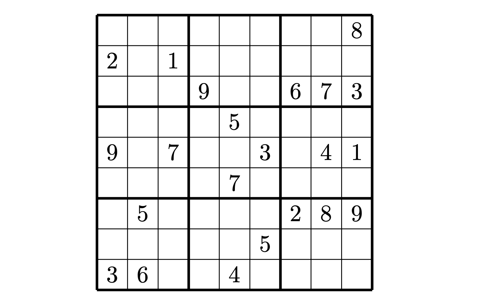
The classic version of Sudoku uses a 9x9 grid, divided into nine 3x3 boxes. Each cell must be filled with a number between 1 to 9. A puzzle begins with some cells already filled in, and your task is to complete the rest - under the following rules:

1. Each row must contain all numbers from 1-9 exactly once.

2. Each column must contain all numbers from 1-9 exactly once.

3. Each 3x3 box must contain all numbers from 1-9 exactly once.

For example, here’s a Sudoku puzzle:

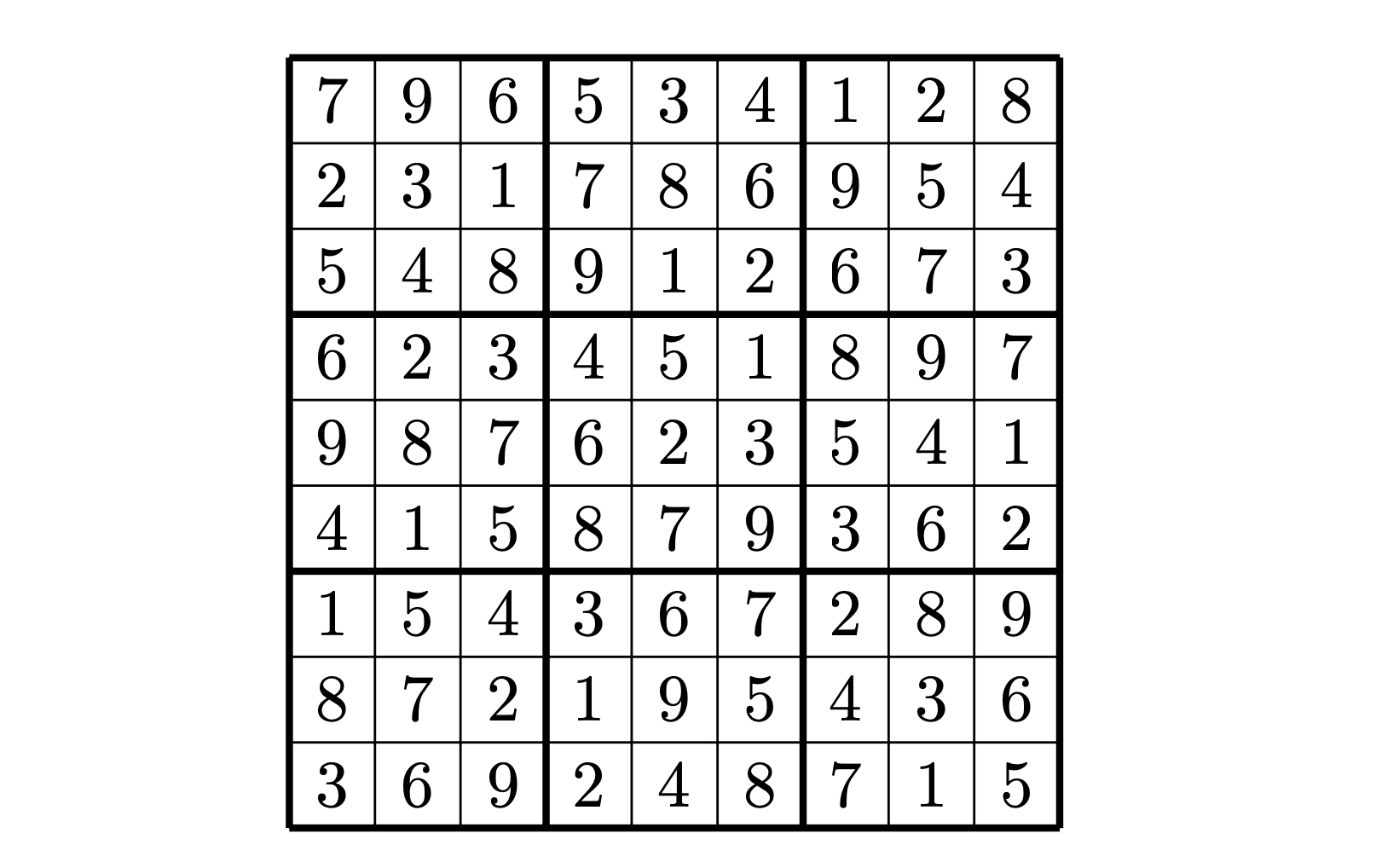
And here’s a possible solution:

Sudoku Solver - Brute Force Solution

If you’ve ever done coding challenges, you might have seen the problem before. In fact, there’s a LeetCode problem dedicated to it: LeetCode 37. Sudoku Solver.

There’s a pretty straightforward way to solve Sudoku - using backtracking.
This is also the approach most people write for the LeetCode Problem.

Here’s the pseudo-code for the algorithm:

01  function solve(cellNum):
02      
03      if cellNum == 81:
04          printBoard()
05          return
06
07      row = cellNum / 9
08      col = cellNum % 9
09
10      if !isEmpty(board[row][col]):
11          solve(cellNum + 1)
12          return
13
14      for digit = 1; digit <= 9; digit++:
15          if canPlace(row, col, digit):
16              board[row][col] = digit
17              solve(cellNum + 1)
18              board[row][col] = 0   # backtrack

The above program prints all possible solutions for a given Sudoku puzzle.
Here’s the step-by-step idea behind it:

1. Go to the next empty cell.

2. Try placing digits from 1 to 9, one by one.

3. If a digit fits (i.e., doesn’t break Sudoku’s rules), move on to the next cell.

4. If you ever reach a point where no digit fit, backtrack to previous cell and try a different number.

5. If you ever reach the end (no empty cells left), you’ve found a valid solution!

Time Complexity and Optimisation Motivation

The brute-force backtracking method will always find a solution if one exists - but it can take a lot of time to do so.

If there are M empty cells on the grid, and each cell can take any value from 1 to 9, the upper bound on time complexity becomes:

\(O(9^M)\)

This can become quite large as M can go up to 9x9 = 81.

In fact, a generalised NxN sudoku is an NP-complete problem. So, in terms of computational complexity, we can’t reduce it to polynomial time - unless someone finally proves P = NP.

But we can make the algorithm faster in practice. Let’s see how.

Sudoku Solver - Algorithm X

Before we start building our solver, let’s first understand what NP-complete really means.

NP-complete problems are a special class of computational problems that share two key traits:

1. Easily verifiable: If someone gives you a potential solution, you can check whether it’s correct in polynomial time (i.e., quickly).

2. Computationally hard: No known algorithm can solve all NP-complete problems efficiently - every known solution can take exponential time in the worst case.

Some well known examples of NP-complete problems include:
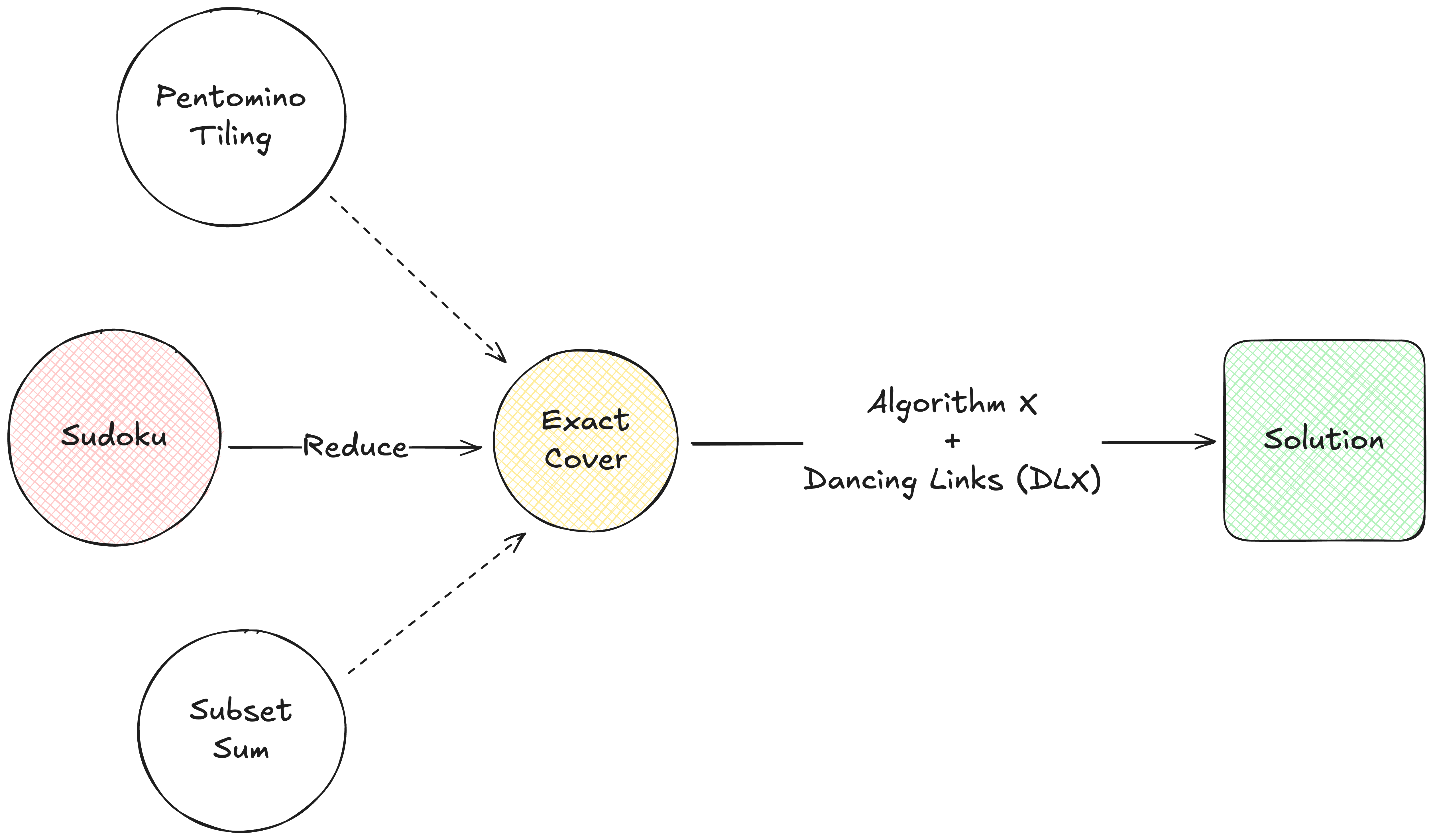
Sudoku (generalised NxN version), Subset Sum, Boolean Satisfiability (SAT), Pentomino Tiling, and the Exact Cover Problem, among others.

A nice property of NP-complete problems is that “any NP-complete problem can be reduced to any other NP-complete problem in polynomial time”.

This means if we can design an algorithm to efficiently solve one of them, we can use it (via reductions) to solve all other problems in the same class.

Note: This also implies that if someone ever discovers a polynomial time algorithm for even one NP-complete problem, it would effectively solve all NP-complete (and NP) problems efficiently - proving P = NP.

Overview

Donald Knuth came up with a nice and optimised approach for solving a classic NP-complete problem called the Exact Cover Problem. He called this backtracking approach, for lack of a better name, Algorithm X. And later he paired it with a smart data-structure called Dancing Links (DLX) to make it blazing fast in practice.

Our solver has two main parts:

1. Reduce the Sudoku Puzzle to an Exact Cover Problem.

2. Solve the Exact Cover Problem using Algorithm X.

We’ll start with the core first - solving Exact Cover using Algorithm X.

Part 1: Solving Exact Cover Problem using Algorithm X

Exact Cover Problem

The Exact Cover Problem, for our purposes, can be defined as follows:

Given a binary matrix, containing 0s and 1s, does it have a set of rows containing exactly one 1 in each column?

This subset of rows will be called the Exact Cover of the original binary matrix.

For example, look at the following Matrix and try to select some rows, such that 1 appears in each column exactly one time.

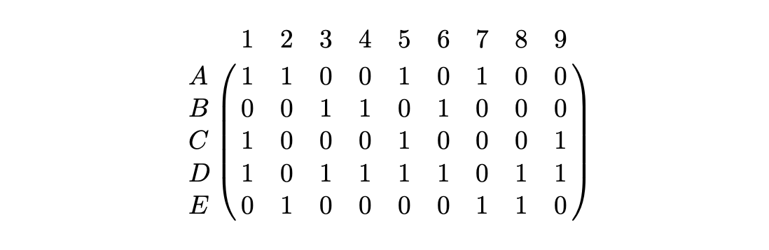
If you look closely, you would find that if you select rows B, C and E, each column would contain exactly one 1.

More formally, if our universal set is S = {1, 2, 3, 4, 5, 6, 7, 8, 9}, then:

• B ∪ C ∪ E would be the exact cover of S (as all columns contain a 1)

• B ∩ C = C ∩ E = E ∩ B = ɸ (as no column contains more than one 1)

A one-liner property we want is MECE - Mutually Exclusive, Collectively Exhaustive.

We want to select the rows which do not have any column in common, but together make up for all the columns.

This is a generalised problem and many problems can be reduced to the Exact Cover Problem including Sudoku. We can imagine the columns to be the constraints, where each constraint should be satisfied exactly once. We can imagine the rows as the decision space, where we can take some rows to form our solution. This is discussed in-depth when we convert Sudoku to Exact Cover.

Algorithm X

Algorithm X is a nondeterministic algorithm that finds all solutions to the Exact Cover Problem. It is simply a brute-force backtracking approach, done in a slightly different manner. The real optimisation comes from how we are able to efficiently implement this algorithm (using Dancing Links). As Knuth states it:

“Algorithm X is simply a statement of the obvious trial-and-error approach. (Indeed, I can’t think of any other reasonable way to do the job, in general.)“

Let’s look at its steps, as given by Knuth in his research paper. Given a matrix A:

from Dancing Links (Donald E. Knuth, Stanford University)

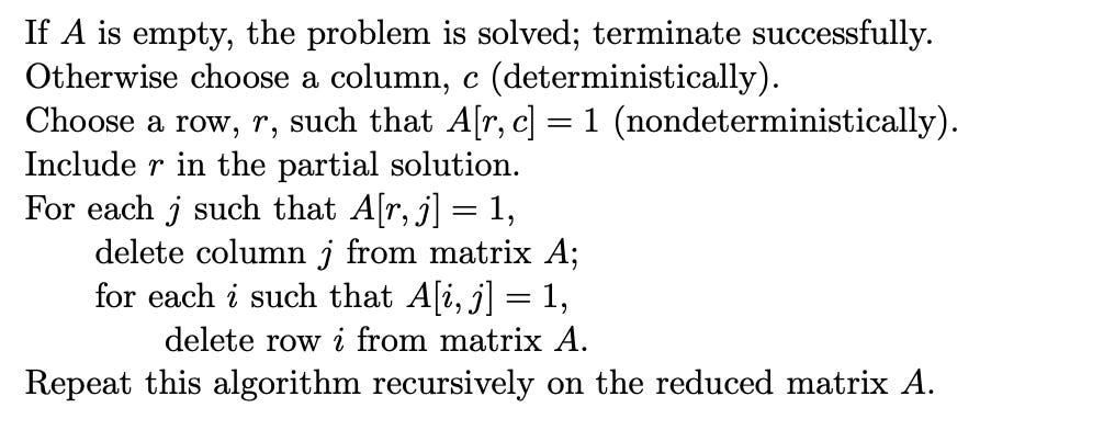
Explanation

Given a matrix A, with 0s and 1s:

1. If A is empty, we’ve found a solution → Base case: terminate successfully.

2. Otherwise, choose a column, c → any column will do, though a smart heuristic (like picking the one with the fewest 1s) makes things faster.

3. Choose a row, r, such that A[r, c] = 1 → basically means choose a row which has a 1 in the column c. ”Nondeterministically” here means try all possible rows, one by one, via backtracking.

4. Include r in the partial solution → this is our current set of chosen rows that might form a valid exact cover.

5. For each j such that A[r, j] = 1 → each column that has 1 in the row r.

   1. delete column j from matrix A

   2. for each i such that A[i, j] = 1 → all rows with a 1 in that column j

      1. delete row i from matrix A.

6. Repeat this algorithm recursively on the reduced matrix A.

7. Backtrack - undo your last choice, and choose another row.

Tip: Try doing a dry run of the above algorithm using a pen and paper, of the binary matrix shown earlier. You can also make your own matrix and watch how rows and columns disappear step-by-step to internalise the process.

If we summarise Algorithm X in the simplest possible way:

1. Pick a column c (randomly, or using some other logic).

2. Try picking rows which have a 1 in that column.

3. After picking a row, say r, include it in the solution.

4. Remove all the columns which have a 1 in row r (as we now have a 1 in those columns).

5. Also, remove all the rows which have a 1 in those columns (as we need exactly one 1 in those columns).

6. Now try solving the same problem on the reduced matrix, using recursion.

7. Once you come back from recursion, undo your selection, i.e., remove the row r from solution, and undo all the operations you did (removal of columns and rows).

8. Again try picking a row from column c.

9. If you ever reach a state where the matrix is empty, you have a solution - which is the solution set you have maintained till now.

Some of you might have noticed that this is just “backtracking with extra steps”. And that is actually true. The real optimisation comes from the fact that we will be able to implement this algorithm quite efficiently - using Dancing Links.

Dancing Links (DLX)

For some time, forget about our original problem, and focus on a technique that Donald Knuth calls

“…an extremely simple technique that deserves to be better known.”

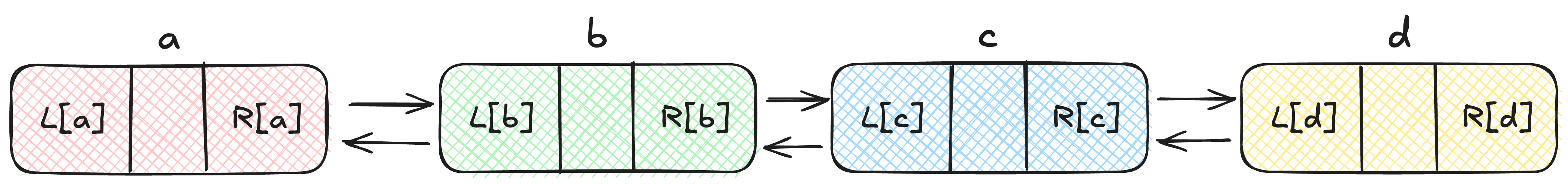
Imagine a Doubly-Linked List.
Suppose x points to an element in that list, and let L[x] and R[x] be the predecessor and successor of that element. Now to delete x from the list, we can do:

\(L[R[x]] = L[x], \qquad R[L[x]] = R[x]\)

This is pretty straight-forward. Setting the left pointer of the right node to the left node, setting the right pointer of the left node to the right node, would remove the node x from the linked list. But comparatively few programmers have realised that the subsequent operations:

\(L[R[x]] = x \qquad R[L[x]] = x\)

will put x back in the list again. This is the operation that Knuth thinks is not well-known. This insertion works because x still has the references it had, before it was removed from the linked list.

The beauty of this operation is that it can undo the deletion operation by just having the references of x and nothing else. Usually, we tend to delete the node and free-up memory once we remove a node from the linked list. But keeping the pointers of nodes intact has surprising benefits in backtracking programs. We can re-insert a node in the linked list (undo the deletion) by just having a pointer to it.

But be careful, if you dry-run this on some examples, you would realise that you cannot just delete nodes and insert them back in any order. For this to work, you can delete a sequence of nodes, and insert them back in the reverse order as they were deleted.

Look at the following example:

A double-linked list with 4 nodes

If we delete the node b, it would look like this:

After deleting node “b”

Now, if we delete node c:

After deleting node “c“

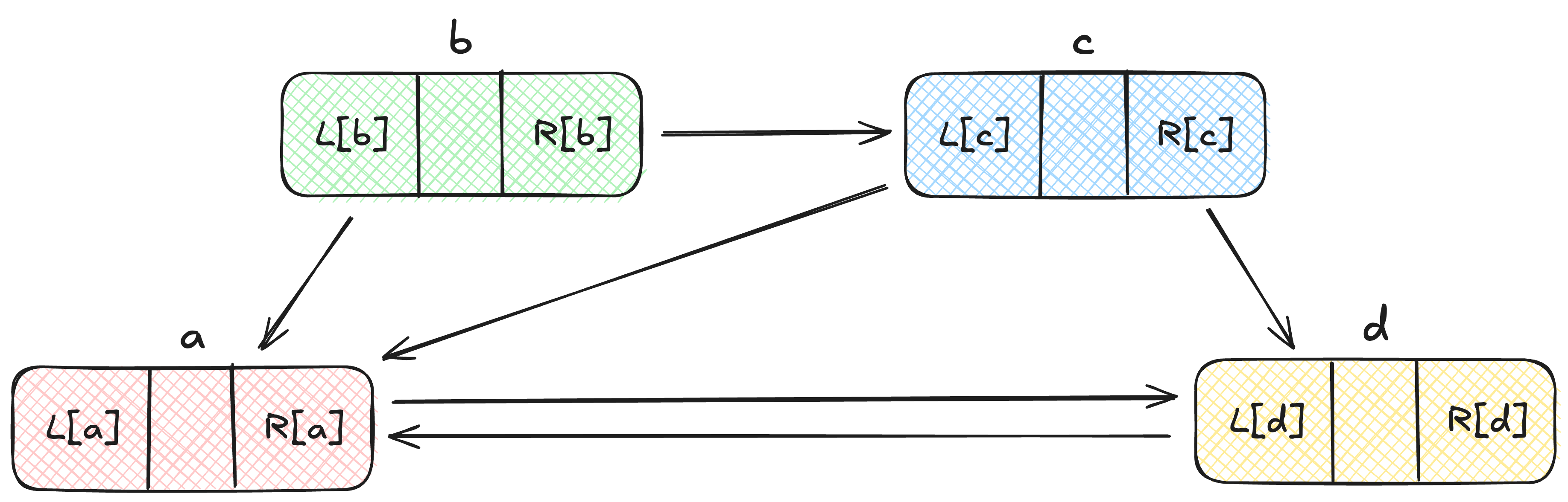
Now you would realise that we cannot simply add node b back again using the operations we discussed, it would leave the linked list in an inconsistent state. We need to first add back c, and then we can add back b.

Therefore, we come to the conclusion that this technique of adding back nodes in a doubly-linked list works like an undo operation - which is perfect for our backtracking program.

The Dance Steps

Now that we understand the basic idea of Dancing Links, let’s look at the data-structure and operations we’ll use to implement Algorithm X efficiently.

We’ll represent our binary matrix as a collection of interconnected nodes, where each 1 in the matrix corresponds to a node (we don’t create nodes for 0s).

Each node x will have the following fields:

L[x], R[x], U[x], D[x], and C[x].

Each row and column in the matrix is represented as a circular doubly linked list, where:

1. L[x] → points to the previous node in the same row.

2. R[x] → points to the next node in the same row.

3. U[x] → points to the node above in the same column.

4. D[x] → points to the node below in the same column.

Each column list also has a special header node, which stores information about that column. C[x] points the column header node of x.

We also maintain a field S[x] on each column header - representing the number of nodes in that column (i.e., how many 1s are present)

---

Note: Since all lists are circular:
1. The last node in the list points to the first node.
2. If a list has only one node, the node’s pointer refer to itself.

---

You can imagine this structure as a grid of linked lists, connected horizontally (rows) and vertically (columns), sharing nodes at intersections.
Each column has a header node at the top, and all column headers linked together, forming a top-level list that serves as the entry point into the structure.

To access the entire structure, we’ll keep a root node, which links to the column headers.

Tip: It’s also useful to keep two additional fields on each node - the row number and column number - to make implementation easier later.

For example, given the following binary matrix:

\(\begin{pmatrix} 0 & 0 & 1 & 0 & 1 & 1 & 0 \\ 1 & 0 & 0 & 1 & 0 & 0 & 1 \\ 0 & 1 & 1 & 0 & 0 & 1 & 0 \\ 1 & 0 & 0 & 1 & 0 & 0 & 0 \\ 0 & 1 & 0 & 0 & 0 & 0 & 1 \\ 0 & 0 & 0 & 1 & 1 & 0 & 1 \\ \end{pmatrix}\)

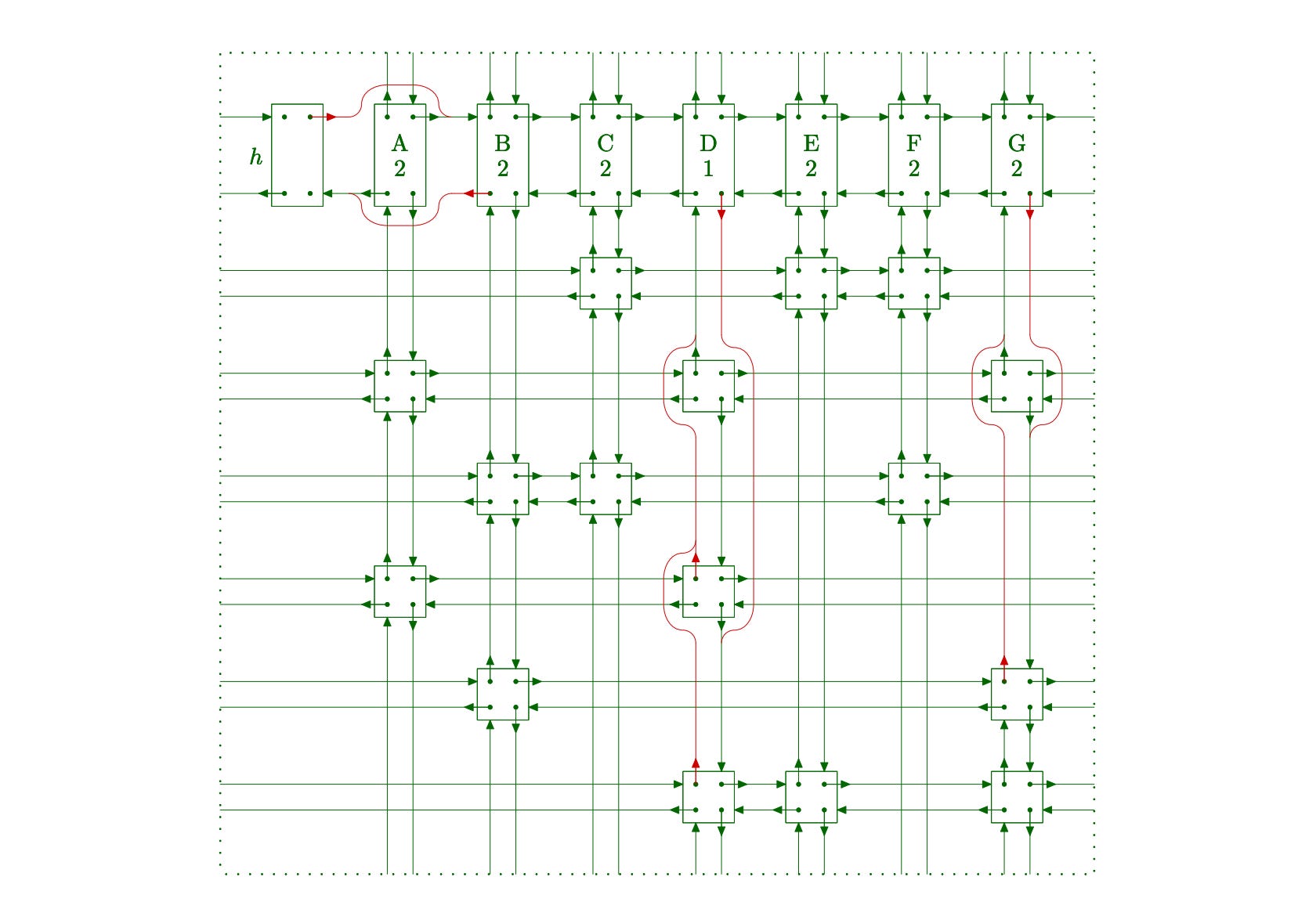
The corresponding DLX structure would look like this:

Four-way-linked representation of the binary matrix

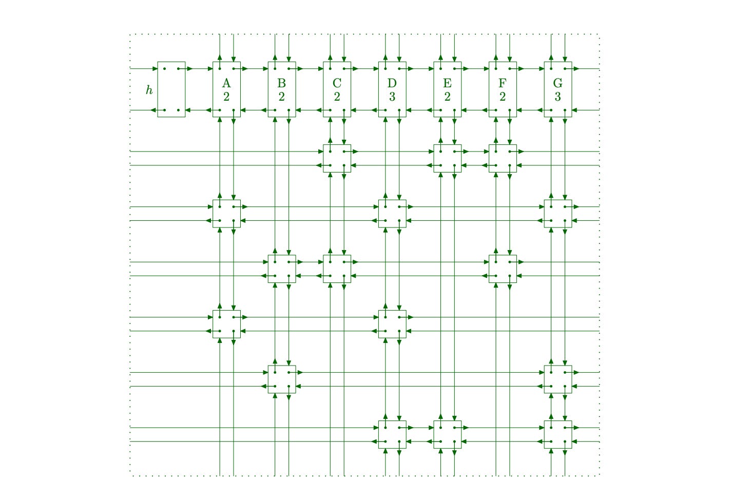
In the above image, h is the root node and {A, B, C, D, E, F, G} is a column header node. Also, C[] links are not shown, but each link would go from a node to the top column node.

Implementing Algorithm X using Dancing Links

Before we jump into the main algorithm, let’s define two important helper methods that we’ll use:

1. Cover: This function takes a column node and removes it from the matrix. While doing so, it also removes all the rows that have a 1 in that column. (since in an exact cover, only a single row can have a 1 in a given column.)

2. Uncover: This function does the exact opposite of cover, as the name suggests. It restores a previously removed column and all its associated rows back into the matrix - effectively undoing the last operation.

We’ll see the implementations of these functions later, for now lets focus on the main algorithm itself.

Let’s define the function “search(root, sol)” where root is the root node and sol is the solution with a list of nodes. The pseudo-code of the algorithm would look something like:

01  function search(root, sol):
02      
03      if R[root] == root:
04          printSolution(sol)
05          return
06
07      col = chooseColumn(root)
08      cover(col)
09
10      for row = D[col]; row != col; row = D[row]:
11          addRowInSolution(row, sol)
12          for j = R[row]; j != row; j = R[j]:
13              cover(C[j])
14
15          search(root, sol)
16
17          for j = L[row]; j != row; j = L[j]:
18              uncover(C[j])
19          removeRowFromSolution(row, sol)
20
21      uncover(col)

Let’s understand what’s happening here, line by line:

Lines 3-5:
We check if there are no columns left in the header list implying all constraints have been satisfied, therefore, we have found a valid solution. So, we print it and return. (How we print depends on the problem - we’ll see that later when we implement Sudoku reduction.)

Line 7:
We choose a column to cover next. This step plays a big role in how fast our algorithm runs. If we simply choose the next column, like R[root], it works fine but is not optimal. Knuth observed that choosing the column with the fewest 1s left gives the best performance. That’s why we maintain the size S[col] in each column header, and also maintain column links for every node. After choosing this column, we cover it.

Line 10:
Now we iterate over all the rows that have a 1 in this chosen column.

Line 11:
We include that row in our current solution.

Lines 12-13:
We then go through all the other 1s in that row and cover those columns, because they’re now satisfied (each contains a 1 in our chosen row). We’ll look at what the cover() function actually does in a bit.

Line 15:
Once we’ve covered all the related columns, we recursively call search() on the reduced matrix.

Lines 17-19:
This is where we backtrack. We uncover all the columns that we previously covered due to this row, and remove the row from our solution. Then the loop continues with the next row in the same column.

Line 21:
After we’ve tried all the rows in this column, we uncover the column itself and return.

Now let’s look at the cover and uncover functions, and how they work.

Cover Function

The cover() function takes a column node and removes it from the matrix. In the process, it also removes all the rows which have a 1 in that column because exactly one row should have a 1 in a particular column.

Try to image how the structure would look after covering a column. For reference, look at the following figure in which red-links are the changed links after column A is covered.

Links after column A is covered

The pseudo-code of the cover function would look something like:

01  function cover(col):
02      L[R[col]] = L[col]
03      R[L[col]] = R[col]
04
05      for rowStart = D[col]; rowStart != col; rowStart = D[rowStart]:
06          for j = R[rowStart]; j != rowStart; j = R[j]:
07              U[D[j]] = U[j]
08              D[U[j]] = D[j]
09              S[C[j]] = S[C[j]] - 1

Line 2-3:
We remove the column header from the column-header list.

Line 5-9:
We iterate over all the rows (nodes) in that column from top to bottom, and remove those complete rows from the matrix, going from left to right. We also decrease the size / count of the column header node whenever we remove a node from that column.

Note: To remove a complete column, we just need to remove its column header from the column header list. Therefore, we don’t actually change the U, and D links of the nodes in the column being covered.

Uncover Function

Once we are done with the cover function, it is quite simple to write the uncover function. By the very nature of the trick that Knuth talks about, we just need to the operations in reverse order to uncover a column.

The pseudo-code of the uncover function would look something like:

01  function uncover(col):
02      for rowStart = U[col]; rowStart != col; rowStart = U[rowStart]:
03          for j = L[rowStart]; j != rowStart; j = L[j]:
04              U[D[j]] = j
05              D[U[j]] = j
06              S[C[j]] = S[C[j]] + 1
07
08      L[R[col]] = col
09      R[L[col]] = col

Line 2-6:
We iterate over all the rows in the column from bottom to top, and restore the complete rows in the matrix, going from right to left. We also increase the size / count of the column header node whenever we restore a node from that column.

Line 8-9:
We restore the column header node in the column-header list.

Note: We must be careful to restore the rows from bottom to top, as we removed them from top to bottom. Similarly, it is important to uncover the columns from of row r from right to left, because we covered them left to right.

---

Task 1: Implementing DLX

We have covered quite a lot of stuff and are done with the first part of the problem. At this point, you should take your time to implement whatever we have covered so far. Write a program, in your favourite language, that:

1. Takes a binary matrix as input

2. Build its corresponding DLX structure

3. Applies Algorithm X on the DLX structure

4. Prints the solution: row numbers of the rows selected in the original Exact Cover Matrix.

For this implementation, you might need the following functions:

1. BinaryMatrixToDLX(): converts binary matrix to DLX structure/

2. ChooseColumn(): selects a column to cover, you can experiment with random selection, or selecting the column with least number of 1s.

3. Cover(): covers the given column.

4. Uncover(): uncovers the given column.

5. PrintSolution(): prints the solution / row numbers.

6. Search(): The main backtracking function of Algorithm X.

---

Part 2: Reducing Sudoku to Exact Cover

Now that we have implemented Algorithm X, let’s see how we can reduce Sudoku to an exact cover problem.

Let’s quickly recall the basic rules of Sudoku:

1. Cell: each cell must contain a single integer between 1 and 9.

2. Row: each row must contain all integers from 1 to 9, with no repeats.

3. Column: each column must contain all integers from 1 to 9, with no repeats.

4. Box: each 3x3 box must contain all integers from 1 to 9, with no repeats.

---

How do we convert these rules into a bunch of 0s and 1s in a matrix?
→ We can do that by treating rows as choices and columns as constraints.

---

Rows as Choices (Decision Space)

We’ll consider each row in the matrix as a possible choice we can make on the Sudoku grid.

For example:

• placing the number 2 on cell (1, 3), or

• placing the number 1 on cell (0, 8)

Each of these represents one possible choice in the puzzle.

Now, how many total choices do we have?

There are 9 x 9 = 81 cells, and each cell can contain 9 possible digits.
That gives us a total of 9 x 81 = 729 choices.

Therefore, our binary matrix will have 729 rows, where each row represents one possible placement (choice) on the Sudoku grid.

Columns as Constraints

Every time we make a choice - say, placing a number 1 in cell (0, 0) - we automatically eliminate several other choices:

• No other number can go in cell (0, 0).

• No other cell in row 0 can contain 1.

• No other cell in column 0 can contain 1.

• No other cell in 3x3 box containing (0, 0) can contain 1.

In other words, by choosing a row in our matrix, we eliminate all the rows that represent invalid options.

How can we ensure that this elimination happens automatically?

By giving these conflicting rows a common 1 in the same column.

In an exact cover, only one row can be chosen for any given column, so rows sharing a 1 in a column are mutually exclusive.

This is how we can represent Sudoku’s constraints using columns in our matrix.

For example, suppose the first 9 rows represent placing the digits 1 to 9 in the first cell (0, 0). If we pick one of these rows (say, placing 5 in (0, 0)), all the others should be excluded. We can achieve this by adding a column in which all these 9 rows have a 1, and all other rows have 0. This guarantees that in an exact cover solution, only one of those 9 rows can be chosen.

Using this idea, we can model each Sudoku rule as a separate set of constraints - each mapped to a different group of columns in our binary matrix.

For the following sections, let’s denote our Sudoku grid as G (0-indexed) and the binary matrix we’re constructing as M.

Cell Constraint

Each cell in the Sudoku grid can take 9 possible values. That means, for every cell, we have 9 candidate rows in our matrix M - one for each possible digit (1-9).

From these 9 candidates, exactly one row must be chosen, since each cell can contain only one number. Also, the choice for one cell should not interfere with the choices for other cells - because, for now, we’re only enforcing the cell constraint.

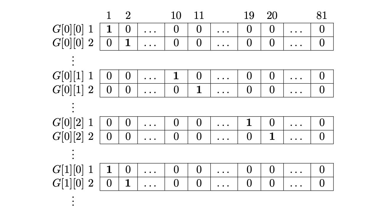
So, the first 9 rows in M corresponds to the 9 candidates of the first cell, G[0][0]. All these rows will have a 1 in the first column of the matrix.

The next 9 rows in M corresponds to the 9 candidates of the second cell, G[0][1]. All these rows will have a 1 in the second column of the matrix.

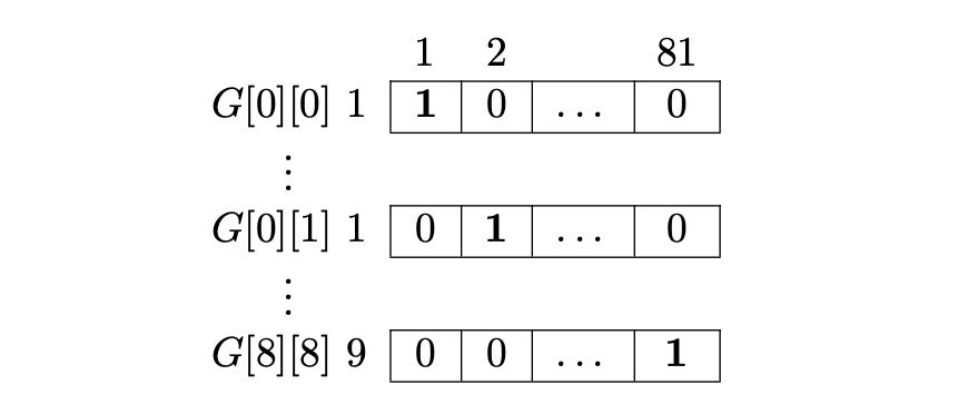
Whenever the algorithm selects a row from the first 9 rows, it automatically removes the other 8 candidates - because in an Exact Cover Problem, each column can have exactly one 1 in the final solution.

This way, we end up with 9 x 81 = 729 rows (representing all possible cell-digit combinations), and we need 81 columns to enforce the cell constraint.

Row Constraint

Each row in G can contain only the digits 1 to 9, each appearing exactly once. To preserve this constraint in M, we’ll arrange the 1s in a different pattern from the cell constraint.

For every row in G, the 9 corresponding cells must collectively satisfy this rule. That means we’ll place the 1s for one Sudoku row in G across 9 separate rows in M.

Each row in the binary matrix M will knock out 8 other rows.

For example, if we place 1 in G[0][0], that corresponds to the first row of M.
Now, all cells from G[0][1] → G[0][8] cannot also have the number 1.

So, all rows in M that represent placing 1 in any of those cells (G[0][0] to G[0][8]) will share a 1 in the same column - ensuring that only one of them can be chosen.

We apply the same idea for all digits 2 → 9 in the first Sudoku row, and similarly for every other row in G.

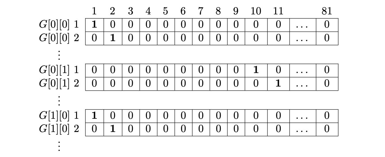
So, the rows in matrix M are arranged as follows:

Rows 1, 10, 19, 28, 37, 46, 55, 64, 73    -> 1 in column 1  
Rows 2, 11, 20, 29, 38, 47, 56, 65, 74    -> 1 in column 2  
...  
Rows 9, 18, 27, 36, 45, 54, 63, 72, 81    -> 1 in column 9  
Rows 82, 91, 100, 109, 118, 127, 136, 145, 154 -> 1 in column 10  

…and so on, continuing this pattern up to the 81st column.

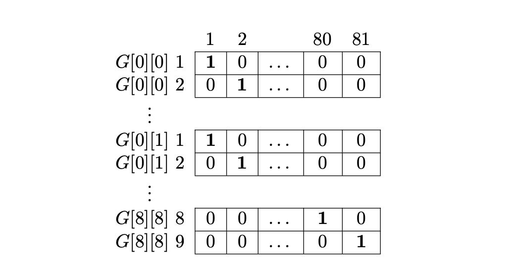
We add this row constraint alongside the cell constraint, giving us a matrix M of size 729 x (81 x 2) = 729 x 162.

Column Constraint

Just like rows, each column in G can only contain the digits 1 to 9, each appearing once.

The first row in M represents the choice G[0][0] = 1.
If that’s true, then G[1][0] cannot also contain 1 - that corresponds to row 82 in M. Similarly, G[2][0], G[3][0], …, G[8][0] also cannot contain 1, which correspond to rows 163, 244, and so on.

This pattern repeats for every column in G and for every digit from 1 to 9.

Just like before, we put a 1 in the same column in M for all the choices that are mutually exclusive. For example, since G[0][0] = 1 and G[1][0] = 1 cannot both exist in a valid Sudoku (due to the column constraint), both rows in M share a 1 in the same column - forcing the algorithm to choose only one.

If you try to draw this pattern on paper, you’ll clearly see the pattern being formed. This will make it much easier to implement this pattern in code.

Box Constraint

Finally, each 3x3 box in G must also contain the digits 1 to 9, each appearing exactly once.

The first row in M again represents the choice G[0][0] = 1.
If we place a 1 in G[0][0], then:

• G[0][1] cannot also have 1 → corresponds to row 10 in M.

• G[0][2] cannot also have 1 → corresponds to row 19.

• G[1][0] also cannot have 1 → corresponds to row 82.

And so on, covering all the cells in the same 3x3 box.

This pattern repeats for every number from 1 to 9, and for every box in G.

Just like before, we put a 1 in the same column in M for all choices that are mutually exclusive - that is, for all choices that cannot coexist in a valid Sudoku configuration.

---

Task 2: Reduce Sudoku to Exact Cover

Now we understand how we can create an exact cover matrix to model choices and constraints in Sudoku.

Write a program that creates an Exact Cover Matrix of an empty Sudoku grid, keeping the cell, row, column, and box constraints in mind.

Note: the matrix should be of size 729 x 324.

---

Part 3: Flow of Code and Generating the Solution

We’ve done so much work with linked lists and matrices that it’s easy to lose sight of our real goal: we’re given a partially filled Sudoku grid (a 9x9 matrix), and we need to find and print its completed 9x9 solution.

So, let’s outline the overall flow of our code:

1. Take input: Start with a 9x9 Sudoku matrix (the puzzle to solve).

2. Build the Exact Cover matrix: Create the binary Exact Cover matrix for an empty Sudoku (nothing filled in).

3. Convert to DLX structure: Transform the Exact Cover matrix into our Dancing Links (DLX) structure.

4. Modify the DLX: Adjust the DLX according to the filled cells in the input Sudoku by explicitly choosing the rows corresponding to those fixed values and including them in the solution space.

5. Run Algorithm X: Execute the recursive search until it hits the base case (i.e., a valid exact cover is found).

6. Generate the Sudoku solution: Once a solution is found, convert the chosen rows back into a 9×9 Sudoku grid and print it.

If you’ve followed along so far, then Steps 1-3 are already complete - we’ve written the functions to build the Exact Cover matrix and convert it into a DLX structure.

Now, let’s talk about Step 4, where we modify the DLX based on the Sudoku input.
This step is straightforward:

• Traverse the Sudoku grid and find all pre-filled cells.

• For each filled cell, determine which row in the Exact Cover matrix it corresponds to. For example, if the Sudoku has a 3 at position (0, 0), that corresponds to row 3 in the DLX.

• Next, we need to include this row in our current solution:

  • Push it into our solution set.

  • Traverse that row in the Exact Cover matrix to find the first column containing 1.

  • Using that column, traverse the same row in the DLX structure and cover all columns that contain a 1.

  • This effectively removes the corresponding row (and its conflicts) from the DLX structure.

That completes Step 4 - our DLX is now modified to reflect the initial Sudoku setup.

We’ve already implemented Step 5, the Algorithm X search.

So, let’s move to Step 6, where we convert our solution set into a final Sudoku grid.

The idea here is beautiful and simple:

• First, sort the solution set / array by row numbers.

• Then, traverse the sorted set / array and print ((row number % 9) + 1) for each element.

Why does this work?

Because once sorted, the vector represents all Sudoku cells in order - from G[0][0], G[0][1], … up to G[8][8]. Each cell had 9 possible rows in the Exact Cover matrix (one for each possible digit), so ((row number % 9) + 1) directly gives the actual digit for that cell.

Finally, print these values in a 9x9 format, from left to right and top to bottom - and congratulations, you’ve just built a fully working Sudoku solver using Algorithm X and Dancing Links. Hooray!!!

---

Task 3: Joining the components and generating the solution

Complete the code by wiring everything together and printing the final 9x9 grid.

You’ll do two things:

1. Explicitly include preset rows (from the given Sudoku clues) into the solution space and modify the DLX structure accordingly.

2. Print the solution once 81 rows have been selected (i.e., when all constraints are covered).

---

Conclusion

And that’s it - we’ve built a complete Sudoku Solver using Algorithm X and Dancing Links!

Starting from the rules of Sudoku, we reduced it to an Exact Cover problem, implemented Knuth’s elegant algorithm, and watched the puzzle solve itself.

From here, you can experiment with improving the solver:
try different heuristics in the chooseColumn() function - like always picking the first column, or the one with the fewest 1s (Knuth’s original heuristic).
You could even profile the solver on multiple Sudoku puzzles to compare performance.

You can find the references here:

1. Dancing Links - Donald E. Knuth, Stanford University

2. Solving Sudoku efficiently with Dancing Links

3. My LeetCode 37. Sudoku Solver Solution using Algorithm X (DLX)

This marks the end of a beautiful algorithmic journey - where mathematics, logic, and a touch of clever data structuring came together to make a computer dance.

Until next time, have fun and keep learning!